What is the impact of weight initialization on neural networks?

When using an artificial neural network, it may seem that the values of the weights initialized at each layer don't really matter since these values will eventually be adjusted during the backpropagation step. However, in most cases, the initialization of weights can significantly impact the training time and the performance of the model.

In this answer, we will explore some techniques commonly used to initialize weights in artificial neural networks and how these initialized values can negatively impact the training process.

What are some common strategies to initialize weights?

To illustrate the different techniques of weight initialization, we will be using the following neural network with 2 input features: a single hidden layer with 2 nodes and a single output node. The activation functions we'll consider are the 3 most common ones:

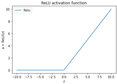
• ReLU

• tanh

• Sigmoid

Convention:

• $w_{j,k}^{i}$ is the weight of a neuron, $b_{j,k}^{i}$ is its bias, and $a_{j,k}^{i}$ is its activation.

• $i$ is the layer in which the neuron $k$ with weight$w$ lies, and$j$ is the neuron in layer $i-1$ whose output is being used as a weighted input to this neuron.

1. Initializing all weights to 0

This naive strategy is widely used by many beginners. However, the wrong approach to follow.

Using the ReLU activation function

When a ReLU activation function is used, the activation $a_{j,k}^{i}$of a neuron is found by$a_{j,k}^{i}=max(0,z_{j,k}^{i})$, where $z_{j,k}^{i}$ is a linear combination of a neuron's weights and inputs.

So, in our example:

$z_{1,1}^{1}=w_{1,1}^{1}(x_{1})+w_{2,1}^{1}(x_{2})+b_{1,1}^{1}$, and

$z_{1,2}^{1}=w_{1,2}^{1}(x_{1})+w_{2,2}^{1}(x_{2})+b_{1,2}^{1}$

However, since all the weights are 0 (including the bias), both $z_{1,1}^{1}$and $z_{1,2}^{1}$evaluate to 0. Thus, $a_{1,1}^{1}$and $a_{1,2}^{1}$are both 0.

Now, if the activations are 0, then during backpropagation, when we update the weights via the following weight update rule: $w_{j,k}^{i}=w_{j,k}^{i}-\eta \frac{\partial L}{\partial w_{j,k}^{i}}$, the partial derivative $\frac{\partial L}{\partial w_{j,k}^{i}}$evaluates to 0, and hence $w_{j,k}^{i}$ never changes and all the weights remain as 0 throughout the training process. Thus, the model never learns anything.

Using the tanh activation function

When a tanh acivation function is used, the activation $a_{j,k}^{i}$of a neuron is found by $a_{j,k}^{i}=\frac{ e^{z_{j,k}^{i}} - e^{-z_{j,k}^{i}} } {e^{z_{j,k}^{i}} + e^{-z_{j,k}^{i}}}$, where $z_{j,k}^{i}$ is a linear combination of a neuron's weights and inputs, as shown above in the case of the ReLU activation function. Here again, $z_{j,k}^{i}=0$. Thus, $a_{j,k}^{i}=\frac{e^0-e^0}{e^0+e^0}=\frac{0}{2}=0$.

As was the case with ReLU, when the weights are updated during backpropagation, they never change and remain as 0.

Using the Sigmoid activation function

When a sigmoid activation function is used, the activation $a_{j,k}^{i}$of a neuron is found by $a_{j,k}^{i}=\frac{1}{1+e^-z_{j,k}^{i}}$, where $z_{j,k}^{i}$ is a linear combination of a neuron's weights and inputs, as shown above in the above 2 cases.

Here again, $z_{j,k}^{i}=0$. Thus, $a_{j,k}^{i}=\frac{1}{1+e^0}=0.5$.

Now, all the neurons in a given layer will have the same non-zero activation value (0.5 in this example). This means that $a_{1,1}^{1}=a_{1,2}^{1}$.

To understand what happens when we update the weights during backpropagation, we first need to look at how $\frac{\partial L}{\partial w_{j,k}^{i}}$is calculated using the chain rule.

$\frac{\partial L}{\partial w_{1,1}^{1}}=\frac{\partial L}{\partial y'}.\frac{\partial y'}{\partial a_{1,1}^{1}}.\frac{\partial a_{1,1}^{1}}{\partial z_{1,1}^{1}}.\frac{\partial z_{1,1}^{1}}{\partial w_{1,1}^{1}}=\frac{\partial L}{\partial y'}.\frac{\partial y'}{\partial a_{1,1}^{1}}.\frac{\partial a_{1,1}^{1}}{\partial z_{1,1}^{1}}.x_{1}$ (1)

$\frac{\partial L}{\partial w_{1,2}^{1}}=\frac{\partial L}{\partial y’}.\frac{\partial y’}{\partial a_{1,2}^{1}}.\frac{\partial a_{1,2}^{1}}{\partial z_{1,2}^{1}}.\frac{\partial z_{1,2}^{1}}{\partial w_{1,2}^{1}}=\frac{\partial L}{\partial y’}.\frac{\partial y’}{\partial a_{1,2}^{1}}.\frac{\partial a_{1,2}^{1}}{\partial z_{1,2}^{1}}.x_{1}$ (2)

$\frac{\partial L}{\partial w_{2,1}^{1}}=\frac{\partial L}{\partial y’}.\frac{\partial y’}{\partial a_{1,1}^{1}}.\frac{\partial a_{1,1}^{1}}{\partial z_{1,1}^{1}}.\frac{\partial z_{1,1}^{1}}{\partial w_{2,1}^{1}}=\frac{\partial L}{\partial y’}.\frac{\partial y’}{\partial a_{1,1}^{1}}.\frac{\partial a_{1,1}^{1}}{\partial z_{1,1}^{1}}.x_{2}$ (3)

$\frac{\partial L}{\partial w_{2,2}^{1}}=\frac{\partial L}{\partial y’}.\frac{\partial y’}{\partial a_{1,2}^{1}}.\frac{\partial a_{1,2}^{1}}{\partial z_{1,2}^{1}}.\frac{\partial z_{1,2}^{1}}{\partial w_{2,2}^{1}}=\frac{\partial L}{\partial y’}.\frac{\partial y’}{\partial a_{1,2}^{1}}.\frac{\partial a_{1,2}^{1}}{\partial z_{1,2}^{1}}.x_{2}$ (4)

So, since $a_{1,1}^{1}=a_{1,2}^{1}$, (1) = (2). Similarly, (3) = (4).

What this means is that when the weights are updated by the weight update rule $w_{j,k}^{i}=w_{j,k}^{i}-\eta \frac{\partial L}{\partial w_{j,k}^{i}}$, $w_{1,1}^{1}$and $w_{1,2}^{1}$are updated the same way (i.e., $w_{1,1}^{1}=w_{1,2}^{1}$after the weights are updated). $w_{2,1}^{1}$and $w_{2,2}^{1}$are updated the same way (i.e., $w_{2,1}^{1}=w_{2,2}^{1}$) after the weights are updated.

This implies two things:

• Since the activations of all the neurons in the hidden layer are the same, the entire hidden layer acts as a single neuron.

• Since all the weights applied to the output of a single neuron remain the same during training, effectively, each neuron has just a single weight coming into it. This means that this model is now linear (and this defeats the purpose of even using a neural network).

2. Initializing all weights to a constant, non-zero value

Whether we use a ReLU, tanh, or Sigmoid activation function, the effect is the same when the weights are initialized to zero with the sigmoid function.

Earlier in our example neural network we saw that:

$z_{1,1}^{1}=w_{1,1}^{1}(x_{1})+w_{2,1}^{1}(x_{2})+b_{1,1}^{1}$ and

$z_{1,2}^{1}=w_{1,2}^{1}(x_{1})+w_{2,2}^{1}(x_{2})+b_{1,2}^{1}$

Now, if $w_{1,1}^{1}=w_{1,2}^{1}$and $w_{2,1}^{1}=w_{2,2}^{1}$, then $z_{1,1}^{1}=z_{1,2}^{1}$. This leads to $a_{1,1}^{1}=a_{1,2}^{1}$and as shown above, this eventually results in the model being unable to capture non-linearity.

3. Initializing weights randomly from a normal distribution

We have seen that choosing a constant value for all the neurons is an incorrect way to initialize the weights. To overcome this, we can choose weights randomly from a normal distribution instead. Each weight is chosen randomly from a normal distribution with a mean of 0 and a variance of 1. While this would solve the problems explained above, this approach also has its caveats.

To see how this can hinder the training, let's consider the following example where all the inputs $x$ are 1.

The weighted sum $z$ will just be the sum of all the weights since all the inputs $x$ are 1.

Now, recall that the mean of the sum of random variables sampled from a normal distribution is the mean of the distribution itself. Hence, the value of $z$ will be a random value from a normal distribution with a mean of 0. However, the variance of the sum of random variables sampled from a normal distribution is the sum of the individual variances, i.e., $v_z=\sum_{i=1}^{n}v_i=\sum_{i=1}^{n}1=n$, where $n$ is the number of inputs and $v$ is the variance.

With the variance of $z$ being equal to $n$ , the value of z is now more likely to be significantly larger or small. When this value gets passed into any activation function, it is very likely to lie in a range where the gradient is close to 0.

In this case, the gradient descent causes very small updates in the value of the weights (barely moving it in the right direction) and thus the network’s ability to learn is hindered and the training time increases drastically.

To overcome the shortcomings of these methods, in 2010, Xavier introduced the Xavier initialization technique for initializing weights.